The Two Spirals Problem Solved Using a simple four-layer perceptron and standard backprop
(You're going to say I cheated.)
While the Two-Spirals Problem may be (or actually, may not be) a valuable
benchmark for neural network researchers working on new architectures, I believe that it
much more valuable, and to a much larger number of people (those working on applied NN solutions), as an example of THE WRONG WAY to present data to a
neural network. This paper is intended as a primer on how to evaluate and
manipulate your dataset prior to building a neural network to improve or
even guarantee your results.
Two researchers, Jiancheng Jia and Hock-Chuan Chua found that
"Using a proper input encoding approach, the
two-spiral problem can be solved with a standard backpropagation
neural network." Well, Duh!
You
can go download their white paper for $35, or read mine for free.
First of all, let me say that I did not cheat.
The whole question of whether I cheated or not, boils down to your
interpretation of the assignment. If you are a student in a classroom, and a
teacher tells you to solve the two-spirals problem (which usually uses x and y
as the inputs) then what I did would be considered “not following directions”
and I’d get a “failing grade” (again, but that’s beside the point).
If, however, you are a professional in any kind of a business environment
working on applied NN solutions, and you’re given the two-spirals problem, then
you have to assume that x and y simply represent the available data, and as a
result, passing x and y through an SQL query in order to turn that data into
inputs that the NN can actually understand isn’t cheating, its simply doing your
job.
In short, you really don’t have to design some ground-breaking neural network
architecture to solve this problem; you just have to understand how an NN
functions, and how the inputs relate (or should relate) to the outputs. (And then
how to modify the inputs accordingly.)
Worst Dataset Ever! This problem is perhaps the best example of bad data for a neural network that I
have ever seen. The authors, I’m sure, were trying to create a challenging
problem, but I don’t think they meant to do this. Because the problem here is
that it’s simply the wrong way to feed data to the NN. There are
several issues with this dataset, all of which are easily correctable.
First, when we (people) look at an x-y plot of this dataset, we see a simple
pattern (the two-spirals). However, when we are looking at that plot, a) we’re
looking at the entire dataset at once (as one fact) and b) we’re using a much
more advanced neural system than any artificial neural network ever invented.
We "input" this one image/fact through a highly specialized neural input device
called a retina. Which is itself an amazing complex grid of neurons responsive
to light and dark (and color), and then we pass that data to the most advanced
pattern recognizer on Earth, the human brain.
Now let’s compare that lovely picture to the actual dataset:
We have chopped up that one image-fact into 194 individual number facts
(pixel-facts?), two inputs each, x and y coordinates (which don’t come close to
occupying the entire x, y plane) coupled with one output; a color (black or
white). In other words, we have turned the act of looking at a picture into
the equivalent of playing the game of Battleship. Think about that for a minute, this dataset does
not represent a picture anymore. To the NN, it’s just, “B-15,” “Miss!” and “A-16,”
“Hit!” over and
over again.
Worse yet, we’re not even giving the computer the benefit of a board and pegs
(because we don’t allow it to memorize the facts). As I have said before, if
you’re going to expect any kind of AI to understand something, you better have
at least one person (i.e. a human brain) who understands it first. I challenge
you to find a single human savant to whom you can call out these x, y
coordinates and “black” or “white” 194 times and have him say at the end, “Oh!
You mean two interlocking spirals!”
So while a summary x, y plot of the dataset has meaning to a person, the
individual facts do not. We can see this a little more clearly when we look at a
line chart of the facts.
(Note: it is my experience that a line chart is a much more reliable method of
showing direct relationships of inputs and outputs. If your facts cannot be
shown clearly on a line chart, it is doubtful you will be able to create an MLP that understands them.)
This line chart looks like the sound wave created by a
guitar string, but that' the only pattern I see. More importantly, there seems
to be no relation between the height of the purple and blue lines (x and y) and
the zig-zagging yellow line beneath (the output).
The other issue with using x, y coordinates as an input is zero. On the x, y plane 0,
0 (“the origin”) is just another point. But to a neural network, zero, as an
input, is nominal. It’s not a number (yes, I know zero is a number) but to a
neural net it represents the absence of input, numbness if you will. Neural
activity decreases as the inputs approach zero (literally, the output of that
neuron becomes zero). But in the two spirals problem, the frequency of the
black/white shift increases as the inputs approach zero, which is completely
contrary to any kind of sigmoid transfer function (which outputs 0 for the input
of 0).
But, now I hear you say, other
people have already solved this problem using more advanced NNs. True. But all
those who have done so, ended up using some form of grid of neurons (i.e. a retina) but they put them in the hidden layers.
Cascade Correlation (Falman and Lebiere, 1991) adds neurons one by one, linking each neuron to all of
the inputs and outputs and to all the other neurons (forming a grid). Alexis Wieland of MITRE, who invented this problem, solved it using quickprop
(Falman 1988) and a network with
five hidden layers of five neurons each, but all the hidden layers were connected to both inputs, again
this forms a
grid.
So I figured that instead of using a hidden-layer grid, the problem could be
more directly solved by using an input grid and a regular multilayer perceptron.
My theory being that this would more closely resemble the retina-brain
relationship, and just might work. The question was, how to arrange this grid,
and many (or actually, how few), neurons I needed. The next step was to take a
really good look at two spirals.
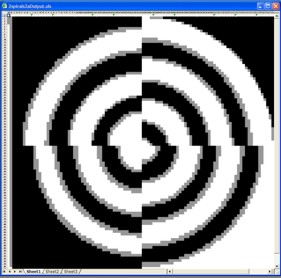
I generated a two spirals image in a photo-editing program by taking black and
white halves and applying a “spiral distortion” of two and a half revolutions,
I then used a pixelization filter to reduce the number on inputs. While a spiral image begins to appear in as few as
100 pixels (i.e. inputs) it takes over 1000 pixels to clearly show the center.
While our eyes are certainly more complex, I figured that 1000 input neurons
were simply too many, and there had to be a simpler solution.
(These animations
are supposed to loop, but on some browsers, you may have to right-click and
"rewind" and then "play" to see them from the beginning.)
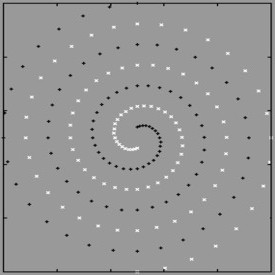
Then I noticed that the photo-editing program’s pixelization filter had another
setting, something it called, “radial pixelization” (which sounded to me like an
oxymoron) so I gave it a try. See the next animation. No matter how few radial
segments I used, the spiral was still clear.
It was now obvious that the
relevant data to this problem was not the x, y coordinates, but rather the
distance from the center point, and the radial location (i.e. bearing) from the
center point. It now seemed almost silly that we were trying x, y inputs in the
first place, we were literally trying to describe a spiral using nothing but
squares (Euclid, please!).
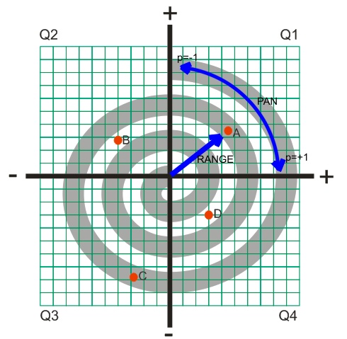
Converting Data to Inputs
I now decided that my input-retina would consist of four neurons, one for each
quadrant, and the value of the input would be the range from the center point.
The means that if our x, y coordinates are +.3, +.4 then our point is in
Quadrant 1 (the q1 neuron), the value is .5 and the other three inputs would be
zero.
This was the same as simply asking the NN to remember that Quadrant 1 is
“black-white-black” and Quadrant 2 is “white-black-white.” I could now say to
you, “Quadrant 1, range 1” and you would respond “black,” and I’d say, “Quadrant
2, range 3,” and you’d say “white.” Even I can remember this!
I also thought the NN needed to know where the point was, within the quadrant,
along the arc at that range. So I designed a fifth input I called “pan” (as in
to pan left and right). This was another simple derivative of the x, y
coordinate, calculated by subtracting the absolute value of x from the absolute
value of y. This number becomes -1 as your point approaches the y axis, and +1
as your point approaches the x axis. It is zero if your point lies on a 45
degree angle from the center point, (i.e. x=y).
A simplified spiral drawn in an illustration program showing how the data was
converted,
see the table below for the resulting inputs from these points.
Original Data
Derived Inputs and Output
Point
X
Y
Color
Q1
Q2
Q3
Q4
Pan
Output
A
0.45
0.35
-1
0.570088
0
0
0
0.1
-0.95
B
-0.4
0.275
1
0
0.485412
0
0
0.125
0.9375
C
-0.275
-0.775
-1
0
0
0.822344
0
0.5
-0.75
D
0.3
-0.3
1
0
0
0
0.424264
0
1
*Note: Points shown are accurate to
the simplified illustration above
and are not actual facts from the two spirals dataset, but you get the
idea.
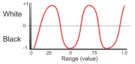
I imagined this would be like putting four optical sensors (or as neurons, rods and cones)
behind a plastic Fresnel lens. If I shined a light at one point, an entire
ring of the lens would light up, but mostly in on quadrant.
Now in my thought experiments, I would have a set of four input neurons each of
which should
respond something this waveform above. I also figured each of these neurons would
be most accurate in the middle of its "optical area" at the 45 degree line, where
pan = 0, and x=y.
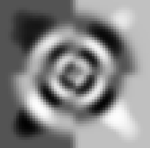
And so I guessed that the total output of the NN would look something like
this illustration (if you squint at it, its a spiral).
It would turn out that I grossly overestimated the amount of generalization I
could get out of this dataset.
It's not
all Black and White
It was to now time to begin experimentation. I wrote an SQL query to convert the
two-spirals dataset (or any other set of x,y coordinates) into the inputs I just described, and I fired up Brainmaker.
My first experiment was just to see if I could train a NN to understand Quadrant
1. My inputs were the q1 neuron and the pan value, the dataset was reduced to
just the points within Quadrant 1. This NN did not train.
So I took a good look at the dataset in Excel (why do I always wait until
after the dataset doesn’t train to do this?).
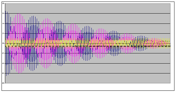
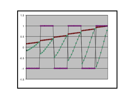
The dataset for he first experiment, Q1 in Red,
Pan in Green, Output in purple.
As you can clearly see, the pan value
was entirely moot. As a matter of fact it's quite distracting even to look at. While you and I can easily ignore irrelevant input, it would
take an NN a million or so training epochs to finally grind all those weights to
zero, and mathematically ignore the input. So I deleted the pan value and tried
again.
This NN almost immediately got about half of the facts right, but then bottomed
out. Back to Excel, where I finally noticed the third and final problem with the
two-spirals dataset, the outputs.
The instructions are to use sigmoid units and
that the network should generalize. But there is absolutely no indication of how
it should generalize.
The outputs are all either black or white, and now that I’ve grouped them by
quadrant, in large groups of black and white, with almost no space between them.
This is a square waveform and not the not the nice curvy sine wave I had
imagined.
The example outputs of the dataset (-1 or +1) are all at the extremes, at the
maximum and the minimum, without a single example of the mean. How do you expect
the NN to generalize when you don’t give it any hint as to where “gray” is, or
for that matter that gray even exists? This also creates an incredible step-size
problem, (which is common in MLPs with bad data).
I
tripped over the Step-Size Problem
The Step-Size problem is basically the problem that
as you adjust the output of any given neuron, (i.e. correcting it because it was
"wrong") if you adjust it too much, you may make the neuron become wrong on
similar inputs that used to be right. That is to say, if .2 is black, .3 is
black, .4 is black, .5 is black, and your asking the NN about .6, its going to
say "black." But the backprop algorithm is going to say, "No, white." and
adjust all the neurons accordingly. But if the Learning Rate is too high,
the NN may now will think that .5 is white too, or at least gray, and most likely
screw up .4 as well.
On the other hand, if the
learning rate is too low, it won't make a large enough adjustment and it won't
be able to adjust the NN far enough to make .6 white, not in one epoch anyway.
And so it will still take forever to train the NN which is just as bad.
Given
the square wave we are asking for as output in this problem, the learning rate
would have to be almost zero in order for .33333335 to be black and .33333336 to
be white. And with that kind of learning rate it would take millions
of years to train that NN with standard backprop. (That's a vast
oversimplification that doesn't take into account the "local minimum" issue, but that
doesn't apply here.)
Anyway the point is that your dataset MUST include at least some "gray."
When we look at the x,y plot
of the dataset, we have ADDED gray to it. indeed the vast majority of the image
is gray. In my thought experiments, I had realized that my quadrant based
neurons would be most accurate along the 45 degree lines and less accurate as
you approach the x or y axis. I had assumed those areas would be gray.
Now I decided that I had to
demonstrate to the NN that we are less confident about the points
closer to the axes. That would mean reducing the output values,
bringing them closer to zero, (i.e. grayer). I
realized that my (then unused) "pan" value was almost perfect for this function. I
subtracted one-half the absolute value of pan from the output if the output was
positive, or added the same amount if the output was negative.
This means that if a given
point lies directly on an axis, its output was now either -.5 or +.5, instead of
-1, or +1. It also means that almost none the points in the data set are now
black or white, (only the ones lying directly along the 45 degree angles), and
almost all of the points are some shade of gray. Also by moving all the output
points off the max and min, we've shown the NN that there is indeed a mean
in there somewhere. And we've created some much needed distance between max and
min, thereby avoiding the step-size problem.
It is also worth noting that while almost all the training outputs are now "gray," they're still
all well within the "40-20-40 Rule" for determining binary output from a sigmoid NN, that is to say: They are all still "correct."
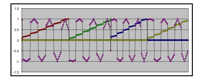
The Little Dataset that Could
All 194 actual derived inputs, Q1 in Red,.
Q2 in Green, Q3 in Blue
and Q4 in Yellow and the final derived
Output in Purple.
You can see the input "range" value increasing from 0 to 1 in each quadrant. You can see a clear direct relationship
between the input and the output, and you can see that the output has a curve to
it that is relatively gentle and very predictable.
Armed with this new dataset, I
went back to BrainMaker. I tried several three-layer perceptrons with between 10
and 100 neurons in the hidden layer. In these experiments I learned that using a
decaying learning rate based on the mean squared error was best, that the
minimum learning rate should be very low (around .0001), and I had been having
the best results with about 25 neurons in the the hidden layer. Unfortunately
those "best results" still bottomed out at about 75% accuracy.
I had wrestling with this for
a few hours and was about to give up, at least for the day, when mainly out of
boredom, I clicked the button in BrainMaker that adds another hidden layer.
I usually don't like extra
hidden layers in my perceptrons. I've read, and I had believed, that there is nothing four-layer
perceptron can do that you can't do in three. And from my understanding of the
math, it seemed to me that all you were doing with a four layer perceptron
was just "spreading out" the calculation between the layers, spreading out the
error, and spreading out the backpropagation function. It really didn't seem to
that there was an advantage to do it. But I clicked the button anyway.
The
damn thing trained in under 5300 epochs. I couldn't believe it. I had walked
away from the computer so I really didn't see it happen, (I was playing Crazy
Taxi at the time) but the auto training
stop had gone off, 100% accurate.
I clicked test. 100%
accurate. I clicked it again, it did again. I poured myself a drink.
The next thing I did was to
generate a set of 10,000 x,y coordinates, and run them through the same SQL
query I used on the original dataset, then I ran that through the NN I had just
trained as a verification set. The results are shown here.
I should point out that The
jaggedness you see is simply the result of the my using only 10,000 points
in my verification set, had I used a million or ten million, the curves would
have been much smoother, but Excel has problems with files that large.
I saved the NN, and then
randomized all the weights and tried again. I was able to train several
different 4-25-25-1 networks all to 100% accuracy. Although each of later ones
trained in between 10,000 and 20,000 epochs. (So I may have been a little lucky
with the random weights on that first try.)
The one anomaly that proves it
As you look at the output plot of the verification set, you may notice one
anomaly: The upper right hand corner (i.e. Quadrant 1 where Range is greater
than 1), this area is black, but I'm not sure precisely why.
There were no training facts that indicated the area
should be black. Indeed, there are no training facts at all with a range >1.
I believe that this is a side-effect of the calculations of the other neurons
combined with a complete absence of training facts that contradict it.
In short, its a guess, a digital guess, and
a damn good guess at that. I think this is proof that the NN understands
the two spirals. The thickness of the white line (all right, the
white arc) is correct, and it certainly fits the pattern. After all, what
comes next in the pattern "black, white, black, white, black, white?"
Obviously black. Its perfectly logical. And yet, it has nothing to do with the
dataset.
Conclusions
The good old MLP trained with standard backprop is a lot more powerful
than most people believe.
You must evaluate the dataset on a fact by fact basis and
not some summary
graphical basis that requires higher brain function to understand.
You (as a person) must be able to understand the relationship between the
inputs and the outputs (on a fact by fact basis) and try to find the most
efficient and logical way to present that data to the NN before you begin
training.
There must be "gray" in the output of the training set.
A four-layer MLP can indeed learn a pattern that a
three-layer MLP cannot.
APPENDIX 1
Why this wasn't cheating
Each "derived fact" was a direct mathematical function of exactly one
"available data fact" and contained no other information.
Each "derived fact" was simply the result of well established mathematic
principles (i.e. Pythagorean Thorium, or simple addition)
The derivation method (i.e. SQL query) was quickly and easily applicable
to any other "available data" input the NN may encounter at runtime, i.e. any other point in
the x, y plane.
There were exactly 194 facts in my training dataset.
APPENDIX 2
The SQL Query
The Two-Spirals dataset I
downloaded (which I called "fctTwoSprials") used an X,Y grid of plus or minus 6.5 for
some reason. This SQL query takes those X,Y coordinates (divides them by 6.5) and
converts them into the input I describe here.
The inputs required for this query are X, Y, the output
labeled "Pattern," and a random number field, "rnd" for random sorting.
The query then calculates the proximity to the X and Y axes, the range from the
centerpoint, and which quadrant. Then it displays the four derived neural inputs I
used (Q1 through Q4) and my derived output "PatternB."
SELECT fctTwoSprials.x, fctTwoSprials.y, (Abs([x]/6.5)-Abs([y]/6.5))/2
AS Prox, IIf([Pattern]>0,[pattern]-Abs([prox]),[pattern]+Abs([prox])) AS
patternB, IIf([x]+0.0001>0 And [y]+0.0001>0,1,IIf([x]+0.0001<0 And
[y]+0.0001>0,2,IIf([x]+0.0001<0 And [y]+0.0001<0,3,4))) AS Quad, Sqr(([x]^2)+([y]^2))/6.5
AS range, Abs([x]/6.5)-Abs([y]/6.5) AS ProxY, IIf([quad]=1,[range],0) AS q1,
IIf([quad]=2,[range],0) AS q2, IIf([quad]=3,[range],0) AS q3, IIf([quad]=4,[range],0)
AS q4, fctTwoSprials.[rnd] FROM fctTwoSprials ORDER BY fctTwoSprials.[rnd];
(Its not exactly an elegant solution, I should have been
able to figure out which quadrant without using a series of four nested "IIF" statements,
but it works.)
Note: There are a few points that lie directly on
the axes. So the query above adds .0001 to each coordinate to "goose" those
points into one quadrant or another. That's the [x]+.0001 stuff you see. I ONLY
do that when determining which quadrant. I don't actually change the x,y
coordinate used in the range or prox calculations.
I notice from my web stats that many of
you are looking for the actual "Two Spiral Dataset"
when you find my site, so here it is:
One Last Note:
(In my research I've noticed that there seems to be a large number of apparently
non-native-English-speaking mathematicians who call this "The Two Spiral
Problem." So if you've been Googling "Two Spirals Problem" you may want to drop
the plural and try again.)
Lastly, It has taken me far longer to write this webpage
than it did to actually solve the Two Spirals Problem, on the order of a
magnitude of ten. So I hope you appreciate it, and you learned about the
process of applied neural network design.

 This problem is perhaps the best example of bad data for a neural network that I
have ever seen. The authors, I’m sure, were trying to create a challenging
problem, but I don’t think they meant to do this. Because the problem here is
that it’s simply the wrong way to feed data to the NN. There are
several issues with this dataset, all of which are easily correctable.
This problem is perhaps the best example of bad data for a neural network that I
have ever seen. The authors, I’m sure, were trying to create a challenging
problem, but I don’t think they meant to do this. Because the problem here is
that it’s simply the wrong way to feed data to the NN. There are
several issues with this dataset, all of which are easily correctable.